VISTA gain/read noise

Read noise and gain measurements with each detector listed on a separate row and each column representing a different filter. The results are consistent across the board with the possible exception of  #16 problems and #13 which is quite non-linear.  H and K are not included as the linearity sequences saturated too early to be useful for this recipe.

Readout noise results

#       NB118            Z               Y                 J
1        22.903        22.782        22.791         27.231
2        22.394        26.694        22.007        26.665
3        20.708       24.783         20.186        25.402
4        21.734       25.758         21.145        27.222
5        21.770       25.989         21.586        28.364
6        21.258       25.579         21.504        26.241
7        24.378       23.737         19.814        24.505
8        21.732       26.474         21.853        27.160
9        19.418      18.838         18.401        19.209
10        24.888      24.740         24.280        25.786
11        24.039      23.504         23.543        25.512
12        25.233       24.403         20.398        25.153
13        26.898      29.973         24.128        25.341
14       19.780      19.652         14.989        20.558
15       17.113      19.643         16.650       17.380
16        23.477      19.398        17.497        22.714

Gain results

#       NB118           Z                  Y               J          Average
1        3.648          3.628           3.630         3.717         3.66
2        4.280          4.251           4.206         4.247         4.25
3        3.957          3.947          3.858         4.045          3.95
4        4.154          4.102          4.041         4.335          4.16
5        4.160          4.139          4.125         4.517         4.24
6        4.063          4.074          4.110         4.179         4.11
7        3.882          3.780           3.787         3.903         3.84
8        4.153          4.216           4.176        4.326          4.22
9        4.639          4.500          4.396         4.589         4.53
10       3.964          3.940           3.867        4.107         3.97
11       4.594          4.492           4.499        4.876         4.62
12       4.018          3.886           3.898        4.006         3.95
13       5.140          5.728           5.764        6.054         5.67
14       4.725          4.695           4.774        4.911         4.78
15       4.088          3.754           3.977        4.152         3.99
16       5.608          4.634           4.180        5.426         4.96

median gain 4.19 (cf. 4.3 for wfcam)

Effective gain in science products

For individual processed science images the internal gain normalisation done when flatfielding yields data products with the same gain value (the median gain of 4.19) for each detector.  In principle, at least, because stacked pawprint science images are averages, clipped as necessary, the overall effective gain for a dither stacked image is simply the original single image gain multiplied by the number of images used in the stack.  Complexities arise because not all stacked image pixels were made from the same number of sub-components (e.g. due to dithering or clipping rejection)  and this is further muddied by the necessary interpolation used in dither stacking.  This latter leads to correlated pixel noise with, in general, a spatially variable noise covariance matrix across each stacked detector image.  For tile images both issues are also present, only more so, compounded even further by the complex pattern of sub-images forming the tile, plus the global reinterpolation of the pawprints to a tangent plane projection.  The associated confidence maps encode the complexity of the pattern caused by the effective number of exposures but not the subtleties introduced by the pixel interpolations.

Sensitivity from flats

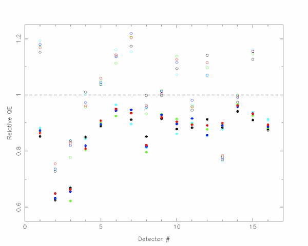
The following figure shows the internal gain as calculated from the flats (open circles) and the sensitivity derived (filled circles) using the gain from the table above (Z: cyan, Y: black, J: blue, H: green, Ks: red).

The internal gain as derived from the flats is provided in the following table which for each chip and filter gives the median value of the flat and its mean absolute deviation in parenthesis.

| Chip  |       Z       |       Y       |       J       |       H       |      Ks       |
|   1   | 1.193 (0.013) | 1.152 (0.004) | 1.180 (0.015) | 1.174 (0.015) | 1.168 (0.002) |
|   2   | 0.735 (0.010) | 0.728 (0.029) | 0.736 (0.015) | 0.755 (0.007) | 0.755 (0.012) |
|   3   | 0.837 (0.032) | 0.836 (0.023) | 0.820 (0.036) | 0.778 (0.018) | 0.829 (0.011) |
|   4   | 1.003 (0.012) | 1.010 (0.028) | 0.973 (0.009) | 0.956 (0.010) | 0.961 (0.012) |
|   5   | 1.039 (0.032) | 1.037 (0.027) | 1.045 (0.015) | 1.049 (0.019) | 1.059 (0.015) |
|   6   | 1.161 (0.033) | 1.142 (0.014) | 1.136 (0.018) | 1.113 (0.023) | 1.143 (0.010) |
|   7   | 1.154 (0.016) | 1.174 (0.008) | 1.219 (0.012) | 1.206 (0.005) | 1.204 (0.003) |
|   8   | 0.952 (0.017) | 0.998 (0.011) | 0.956 (0.023) | 0.933 (0.012) | 0.962 (0.019) |
|   9   | 1.002 (0.003) | 0.998 (0.004) | 1.013 (0.005) | 1.016 (0.001) | 1.004 (0.001) |
|  10   | 1.072 (0.002) | 1.094 (0.009) | 1.116 (0.011) | 1.138 (0.005) | 1.126 (0.009) |
|  11   | 0.964 (0.006) | 0.946 (0.045) | 0.981 (0.014) | 0.959 (0.028) | 0.957 (0.019) |
|  12   | 1.069 (0.021) | 1.141 (0.031) | 1.071 (0.007) | 1.097 (0.006) | 1.115 (0.017) |
|  13   | 0.765 (0.017) | 0.770 (0.005) | 0.776 (0.020) | 0.780 (0.022) | 0.784 (0.018) |
|  14   | 0.999 (0.002) | 0.974 (0.004) | 0.991 (0.003) | 1.000 (0.005) | 0.996 (0.004) |
|  15   | 1.161 (0.015) | 1.127 (0.017) | 1.156 (0.011) | 1.147 (0.018) | 1.155 (0.016) |
|  16   | 0.909 (0.002) | 0.874 (0.006) | 0.883 (0.004) | 0.880 (0.002) | 0.890 (0.004) |