Overview plots
These are meant to provide a quick view of the observations which have been processed (see processing status). The default map shows observations performed in any filter; it is possible to select just one filter to view the observations done in that particular band. Combination of fiters (i.e. areas observed in e.g. J and K) is planned for the future.
There is a page showing all the observations done with VST and one individual page for each large programme. Together with the survey progress overview we provide some simple quality control plots: astrometric WCS rms, seeing, zero point and sky brightness.
Queries and Preview
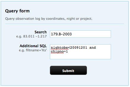
We provide a searchable interface to our quality control tables.
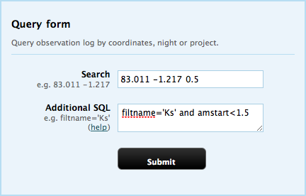
The search term is quite flexible and allows for search on filename, date of observation, coordinate and project. Additionally it is possible to refine the search using the additional SQL box. For example in order to select all images (individual chips) which centre is closer than half a degree to a position we would use 83.011 -1.217 0.5 as the search term. We could refine our search to those images obtained in Ks and in airmass lower than 1.5 by adding the following to the 'Additional SQL' box: filtname='Ks' and amstart<1.5
One can further refine the search to those image which actually contain that position by adding onchip to the search term. Look at the different examples in the search form.
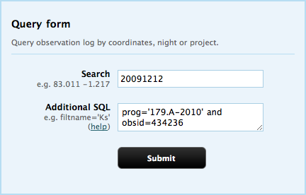
The second example shows how to search for a particular combination of programme, night and observation id (which by the way is not unique). A similar result would be obtained by searching by programme id in 'the Search Box' and adding the night constrain on the 'Additional SQL'.
A full list if SQL column names to use in the additional SQL box is available here.
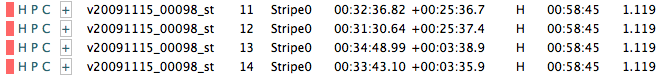
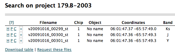
The query returns a list of stacked pawprint images satisfying the criteria. One row per chip is returned with information about object name, coordinates, filter, observation time, zero point, magnitude limit, ...

The first column displays several links to additional information: [H] displays the primary and the selected extension headers, [P] shows a preview of all the chips, [C] shows a preview of the chip with additional QC information, [S] only shows up if searching for a coordinate and the position is in the chip, in which case a finding chart is available. The [+] link expands the row showing additional information like calibration frames used, individual pawprint images which went into the stack and some observation parameters.
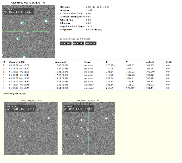
The following image shows an example finding chart which displays the stamp from the stacked image as well as from the individual jitter frames together with the detected objects:
Images are available to be queried as soon as processed and initial checks done on them. We add a red flag to those images which are still subject to change or being reprocessed. You can preview them but you cannot request them.
Nightly QC
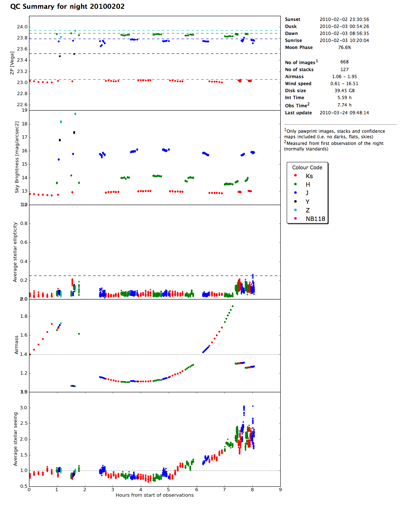
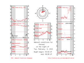
When querying for a night you can view the variation of the zero point, sky brightness, ellipticity, airmass and seeing across the night. There is also a summary of the weather conditions in that night provided by ESO.
Retrieving Data
Only authorized users are able to download VISTA data. CASU provides access to stacked pawprint frames and tiles (calibrated astrometrically and photometrically) as well as individual pawprint images, FITS catalogues and calibration frames. You can login using the link at the top right of the page.
Web Interface
Use the Observation Log Search to search for stacked images. The following examples selects all files for project number '173.B-2003' observed before 20091201 and only displays the first chip.
Once on the results page you can request all data returned by that query following the link at the bottom 'Request these fles'
Insert your username and password and the email you want the instructions to download the files to be sent.

When you click the 'Submit' button you will get a confirmation message and when the download data is ready for retrieval you will get an email with instructions on how to download it.
Note that in order to request data you only need the query ID number. This identifies uniquely all the queries done and it is available at the top right of the query results page. You can get back to any previous query using the query ID or use it to retrieve all data from that query at a later stage as in this example.
You can also create a list of files (see below for the format) and access the request data from here
From The Command Line
- Prepare a file containing the file names to download. The only requirement is that the first column contains the file name of the stacked image. Comment lines starting with the hash character are allowed. Example:
# Filename             Object Name                    Coords
o20111024_00012        ATLAS survey                   23:48:02.57 -12:42:17.6   z_SDSS 1.023 45.00  0.82  0.09  22.43  0.01  0.25  0.9
o20111024_00012_st     ATLAS survey                   23:48:02.57 -12:42:17.6   z_SDSS 1.023 45.00  0.78  0.07  22.43  0.01  0.24  0.9
This file can be obtained by querying the Observation Log and downloading the output table at the bottom of the query result. - Submit your request. Example:
python spvista_request.py -e me@google.com -u username -p password vst_in.asc
Where you need to insert your email address, username and password. The option-tlists the file types to request (by default stacked frames and catalogues). The upload script requires python (2.5 or higher) and can be downloaded here (by authenticated users). - Download your data. You will get an email after the data has been copied to the stage area with instructions on how to download it using wget.
You can request any stacked pawprint, even if it does not belong to your project. The system will automatically detect that you are not allowed to download that data file and will ignore it. Also you can specify the same filename different times (e.g. when listing different chips) so you do not need to clean your input list, but note that you will get a multiextension FITS file with all the 16 chips. There is no limit on the number of files you can request but keep in mind that if you request a stacked image and their associated original pawprint fames you are likeliy to get quite a lot of files (i.e. one stacked image, one confidence map, one catalogue and njitter number of original frames per stack plus flat and sky frames.)
Data format issues
Images are compressed
In order to save disk space and make transferring of images faster we use lossless RICE compression on the images. Most of the modern software deals with compressed images on the fly, e.g. DS9 can preview the images, Python can read them using pyfits as well as all programs based in CFITSIO. If you need to uncompress the images (e.g. if you want to use IRAF) you can use imcopy which is an example C program available from the CFITSIO examples webpage.
Extract magnitudes from catalogues
The catalogues store the flux in counts and the appropriate headers to convert them to magnitudes. The catalogue format and the recipe to compute magnitudes is described in detail in our technical pages. E.g. the magnitude in the aperture number 3 is calculated as:
mag3 = hdr['MAGZPT] - ( hdr['ESO TEL AIRM START'] - 1 ) * hdr['EXTINCT']
       - 2.5 * log10( data('Aper_Flux_3') / hdr['EXPTIME']) - hdr['APCOR3']
We have available a fortran program which converts the FITS catalogues into ASCII. This can be downloaded from the software release page. It needs the CFITSIO library and can be compiled as
gfortran fitsio_cat_list.f -o fitsio_cat_list -L/sw/lib -lcfitsio -lm
and then run as
fitsio_cat_list catalogue.fits
It outputs a file named catalogue.asc with the following columns: RA and Dec coordiantes, x, y, magnitude, magnitude error, chip number, stellar classification, ellipticity and position angle.
Some of the information is only available to registered users. Login here.