Sky subtraction

After the decurtaining step, images are temporally linked to produce master sky frames which are used in the sky correction step. If possible, the sky correction frame is made from the science MSB itself eg. UDS and DXS surveys. If insufficient pointings are available within a single MSB then adjacent MSBs are used to increase the number of sufficiently independent pointings, with the constraint that fields taken within 5 degrees of the Galactic Plane, or centred on bright NGC galaxies, are not used for sky estimation.

The sky frame is formed in a two-stage process. First each dither or interleave sequence is robustly combined (iterative median with upper k-sigma clipping), after first scaling to a common level, to remove the majority of real images. Then a sequence of independent field centres of these intermediate stacks are similarly robustly combined to form the actual sky frame used. In practice, the sky frame is an attempt to correct for mainly additive artefacts including scattered light, residual reset anomaly, and illumination-dependent detector artefacts; although residual flat field errors are also corrected to first order.

Sky correction proceeds by scaling the chosen sky frame, generally the nearest in time to the target frame, to the data and additively applying it, whilst maintaining the original overall target frame sky level.

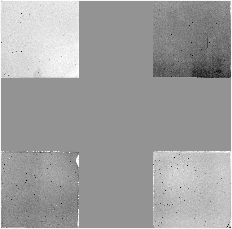
A typical J-band dark sky stack (orientation on-sky with N to the top and E to the left) is shown here and highlights several features of the sky correction.

Residual gradients introduced by the twilight flatfielding strategy are negligible across detectors and are well below the 1% level. The pedestal offsets can be quite large, typically ±4% of sky (it is known they are additive since there are no equivalent photometric systematics). The most variable quadrant on detector #4 also stands out. There is no measurable fringing present in any of the passbands in any of the filters.

Note that sky subtraction is not currently carried out in the summit pipeline.

All sky correction frames are formed from frames matched in passband, readout mode and exptime/nexp.

The various sky estimation strategies that the pipeline now has at its disposal are:

none - not enough data to form a sky so don't bother;
leftovers - odds and sods throughout the night combined to make sky frame;
pawprint - sweaty iterative stacking with ever deeper object masking;
tile - default, usually the best option but needs tile of pawprints
offset skies - there are two modes in use here

• complete offset to nearby region which currently forces the pipeline to use pawprint method to estimate sky due to the way it has been set up
• flipping object/sky between detectors in pairs i.e. 1,2 <-> 3,4 or 1,4 <-> 2,3 this is more effcient since object of interest is always on a detector if it is small enough to fit on one

These strategies are discussed in more detail below.

Pawprint method

For a dither sequence with a reasonable range of offsets there is a good chance that every location on sky is covered by some object-free pixels. Doing a straight forward stack of the images with some form of outlier rejection leads to a good contemporaneous background map providing the jitter offsets are significantly larger than the characteristic size of the point-spread function and no large, or bright objects, are in the field. Where this algorithm fails most often is when the jitter offsets are not sufficiently large to allow the full profiles of the brightest stars to be rejected completely, or when large bright galaxies are present in the field. Bright stellar halos are sometimes only a few percent above the ambient background and hence may not reject out during stacking.

Pawprint method with Object Masking

One way of avoiding the problem of poor rejection of astronomical objects while doing a combination for background estimation is to mask the objects beforehand using the following algorithm:

1. Combine all the object images with rejection to form a sky frame.
2. Subtract the sky frame from all the object images
3. Shift and combine the background-subtracted object images to form a stacked frame
4. Throw away the background subtracted object images
5. Do an object detection on the stacked frame and note where the object pixels are. This forms a master object mask. Note how many object pixels there are.
6. Throw away the stacked frame
7. Recombine the original images with rejection and in conjunction with the object mask form a new sky frame.
8. Go back to step 2. Repeat up to here until the number of object pixels you detect in step 5 roughly converges.

This procedure gives much better results, but with the penalty that it can be quite time consuming because of the repeated object detection and stacking steps. It will still fail in regions where there are no clean sky pixels left after object masking and here the only option is to interpolate between nearby pixels to fill in the gaps. There is a variation on this theme where the algorithm is provided with a mask beforehand. This can be done if the observations are part of a long running project and the mask can be defined by increasingly deeper stacks offline. This method should be quite quick, since the steps above that lead to the creation of the mask (repeated stacking, sky subtraction and object detection) are the main consumers of the computing time. However this approach also implies that any earlier data that were processed using a shallower version of the mask would have to be re-reduced as the mask improves (see also note at bottom of this page re: limitations of pawprint-based methods)

Tile method

If the observations are part of a filled tile, as will be the case with the majority of data, then stacking the separate components that make up a tile is significantly faster and generally gives better results than the pawprint methods. If the observations are part of a tile with M pawprints and each pawprint consists of N exposures then we do the combination in two stages. First we form N intermediate sky frames by combining with rejection all of the input images that are in the ith position in each pawprint sequence (where i=1,M). Because each of these are in vastly different places it is very unlikely that there will be much overlap between objects. We then combine the N intermediate background images with rejection to form a final background image.

Sky flipping

In situations where you have a large extended object and that object is roughly the size of a detector it is possible to use a sky flipping observational technique to allow a sky estimate to be done. The basic idea is that the object is placed on a detector and observed for a full jitter sequence. The telescope is then moved to another position so that the object is now in an adjacent detector and another jitter sequence is taken. A background file is made for each jitter sequence using masked pawprint estimation, but skipping the detector where the object has appeared, resulting in two background files, each with one detector missing. For example, if the object was on detector 1 in the first sequence and then on detector 2 for the second, we use the background estimate for detector 1 in the second sky file to correct detector 1 in the first series and we use the background estimate for detector 2 in the first sky file to correct detector 2 in the second series. This method has the advantage that the object of interest is always being observed and the sky estimate is very close temporally (and spatially) to the object exposures.

Offset Sky Observations

With very large extended sources (i.e. a significant fraction of the field-of- view), the only sensible way to do background correction is with offset sky observations. This is simply done by observing a pawprint, or tile, with the object and then moving the telescope to a point nearby, but far enough away so that contamination by the object or any other large source is not present. This requires no special observing strategy like flipping and only needs a means of associating the two sets of pawprints, or tiles, so that the pipeline knows that they are to be reduced together, using appropriate header keywords. Obviously, both object and sky frames must be observed in the same way (i.e. the same r/o mode, exptime and no. of exposures).

Note on imitations of pawprint-based methods

It is well known that no matter how good the masking algorithm, without an external deeper mask,  sky estimation for single pointings based on a limited number of frames and dithers leaves some residual object flux, below the pixel-level detection limit, in the sky frame.  The residual is diluted by a factor O(1/n) when doing clipped averaging but still leads to oversubtraction of faint outer profile wings by this amount and thereby introduces a small systematic bias which progressively increases at faint magnitudes.

The good news is that for point sources significant differences only arise for heavily saturated objects.  Even for extended sources measured in the default apertures there is very little difference. However, the bad news is that when using Petrosian fluxes, where the extended wings have much more impact, it is a lot worse and the bottom line is that a large fraction of ALL extended sources are noticeably affected. The only way to alleviate this problem is to either use a much deeper object mask as input or to ensure that several pointings, e.g.  a tile sequence, are used for the sky estimate.